Video Processing : Tracking Objects

A video is composed of a sequence of images in rapid succession such that the objects, as you browse through the images, appear to be moving. Thus, image processing can be done on these images by looping through them and applying the same algorithm to each image. 

In commercial cameras, they describe the rate at which a video is captured by fps or "frames per seconds". The most common cameras has 30fps. For this activity, the fps of a Canon 550D is 50. Since the time interval is just the inverse of the frame rate, the time interval between successive images is 0.02 seconds. 

The goal of the activity is to observe the spread of a red dye in water – hot, cold, and tap. The dispersion of the red in water is tracked using color segmentation.

From the last activity, the most effective method for color segmentation is the non-parametric probability distribution estimation. This is done by getting the histogram of a region of interest.  The color we perceive usually varies due to the uneven level of brightness in an object ,thus, the color space used is the NCC (normalized chromaticity coordinates) which separates the chromaticity and color information. The histogram of the ROI (region of interest) represents a blob in the NCC diagram. Through histogram back projection, each pixel location in the image has a corresponding value equal to the histogram value in the chromaticity space. These new set of values make up the image which should show part of the original image that has the same chromaticity as the region of interest.

The figure below shows the area of the red dye when it first touched the water. 

Area of the the red dye as it touched the water 

The red dye was allowed to spread for 30 seconds.  The video was parsed into images using Avidemux with a total of 75 images for processing.

For each image, color segmentation  through non-parametric probability distribution was done. The algorithm was looped through each image.

Histogram and result of segmentation

Plot of the area versus the image number

It can be observed that after 30 seconds, the red dye was observed to spread significantly. In order to quantify its dispersion for the 3 set-ups, the mean and the standard deviation of the area for all the images were computed. The table below shows the mean and standard deviation for the hot, cold and tap water setup.

Mean and Standard Deviation of the Area of Dispersion of  the Red Dye

Among the 3 setups, the red dye spread most widely in the hot water setup. This is due to the fact that water molecules in hot water move faster than in cold water, thus, making the dye spread faster in the medium.

I give myself a 10 for accomplishing the tasks required in this activity. J

References:

1.       Soriano, M., Activity 11 – Color Segmentation.

2.       Soriano, M., Basic Video Processing

Color Image Segmentation

It is difficult to separate colored parts of a color image if it is converted to grayscale then use thresholding for segmentation. Thus, the only approach is to segment the parts by using the color image itself, no conversion needed. However, in the case of objects with differing level of brightness such as 3D objects, it is not advisable to use the RGB space. Instead, one can convert RGB to NCC (normalized chromaticity coordinates). This color space allows separation of brightness and chromaticity. To compute for the values of the red, green and value for NCC, here is the formulae:

This is done per pixel. The sum of r, g and b must be equal to 1. Since b is just equal to 1- r - g, we only use r and g values. The values obtained from using the formula above must between 0 and 1. The chromatic information is stored in r and g while the brightness information is in I.

 In this activity, two approaches were used for color image segmentation - the parametric and non-parametric probability distribution.

I will be working on the image of a flower below. 

Test Image

My goal is to separate the color yellow from the image. The expected result is an image that only shows the parts of the picture that correspond to the color yellow. So, from the image, I will crop a part of the petal. 
The figure below shows the cropped part.

Cropped part of the image (petal)

This is the shade of yellow that I want to separate from the whole image. 

PARAMETRIC PROBABILITY DISTRIBUTION

First, I will get the RGB values of the cropped image and use the equation above to get the correspond r-g values in the NCC coordinates. Then, I will get the mean (μ_r ,μ_g) and standard deviation (σ_r ,σ_g) of the the r and g values. Using the calculated mean and standard deviation, I can get the probability that a particular pixel belongs to my region of interest which is the petals of the flower. The probability is computed by substituting the values of the mean and the standard deviation in the equation below. 

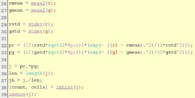
However, the r and g values used in the formula above is the corresponding r and g values of the whole image. The code used to implement parametric probability distribution is as follows:

Code for obtaining the r and values of the cropped image and the whole image

Code for getting the probability that the pixel belongs to the ROI

The result of the color segmentation is shown below. 

Original image (left) and Color Segmentation result (right)

NON-PARAMETRIC PROBABILITY DISTRIBUTION

In this approach, you need not get the mean and standard deviation of the cropped image. You only the histogram of the cropped image. The following two figures show the code for getting the 2D histogram of the cropped image. 

Code for getting the 2D histogram of the image

The 2D histogram of the cropped image must have peak at the point that corresponds to our color of interest if compared to the normalized chromaticity diagram. 

Normalized Chormaticity Diagram (left) and 2D histogram of the cropped image (right)

By estimation, the peak shown in the 2D histogram covers to both the light green and the light yellow in the the normalized chromaticity diagram. Thus, we expect that it will also segment parts of the image that correspond to the light green parts of the image. Using the 2D histogram obtained, we use histogram backprojection to segment the image, leaving only those parts described in the peak of the 2D histogram. 

Code for the Histogram Backprojection

The result of the backprojection is shown below. 

Original Image (left) and result of the histogram backprojection (right)

As expected, it also showed the light green parts. However, comparing the accuracy of the segmentation, the non-parametric probability distribution is better than the parametric probability distribution.

For this activity, I give myself a 10/10 for accomplishing the task at hand. 

I would like to thank Ma'am Jing for helping me understand the concept and for Krizia Lampa for helping me debug the code. :)


Reference:

1. Soriano, M., A11 - Color Image Segmentation 2010

Applications of Morphological Operations Part 3 of 3

Image processing has made it a lot easier to automate naming of parasites in the human blood. Most of the parasites that attack the red blood cells cause the RBCs to have an enlarged shape - bigger than the normal. For example, when a person is affected with malaria, the image below should be seen under the microscope.

Plasmodium vivax

 This one is the case when the parasite present is Plasmodium vivax. It can be observed that the RBCs are larger than the normal.

In this activity, we are given an image of scattered punched papers which we will consider as cells. Th goal is to use all the image processing techniques that we have learned in order to get the area (in pixel count) of the "cells".


First, we are given the image below. The whole image will be cut into 256 x 256 subimage.

Original image

Here is the first sub-image.

1st Sub-image

I first worked on this image. I got the histogram of the image in order to get rid of those that are not cells. 

Histogram of the 1st sub-image

From the histogram of the image, I used SegmentByThreshold () of IPD to isolate the cells. The threshold is at 220. 

Binarized version of the thresholded image

I masked the image above so that we'll be able to isolate the cells. This is the best I can do to separate them. See image below.

Isolated Cells

I used a Bounding Box to emphasize the isolation. However, they were both enclosed in one box. I took the area of this cells inside by taking the length of the pixels which are true in this image and divided it by 2 since there are two circles. I got 510. So for now, this will be my "theoretical" area. This will help me easily filter the other sub-images such that I will only be calculating the isolated cells.

Since I now have a "theoretical" threshold. I will start processing the sub-images. I will use the FilterBySize() function of IPD, setting my SizeThreshold to 510. This means that filter those pixels with sizes less than 510.

To make sure that I am getting the correct area, I have another threshold which I set at 550. Using the same function. this will only show cells greater than the cells of interest. I subtracted the latter image to the former, giving me an image of the cells of interest only. Thus, it is easier for me to know their areas. 

Isolated Cell of Interest

To get the area, we count the number of pixels tagged wit the same number by AnalyzeBlobs () function of IPD. The area of this cell is 517 pixels. I will repeat the same procedure to the other sub-images and tally the area of isolated pixels. The code for getting the area is shown below.


s = length(BlobStatistics);
for i = 1:s
    [area(i)] = length(find(Filt_image1 == i));
end

BE = mean(area);
SD = stdev(area);
disp(area');

However, it was hard to automate the whole process. It was hard to have just one threshold for all the images. So, I have to get the area of the cells for all the sub-images manually.

The best estimate was determined to be 639 pixels with a standard deviation of 485.



ISOLATION OF CANCER CELLS

Another image of scattered punched papers was given to us. However, in this image, the size of the punched papers are not uniform. The presence of bigger punched papers can be attributed to "cancer" cells. The goal of the next part of the activity is to isolate the "cancer" cells n the image and estimate their sizes.

Circles with Cancer

For easy processing, this image was cut into sub-images. Since the 1st sub-image contains a "cancer" cell, I just used to 1st sub-image to accomplish this part of the activity.

1st sub-image of the image with a cancer cell

Using the same procedure as the first part of the activity, the final results is shown below.

Isolation of Cancer Cells

The area of the cancer cell in the image is determined to be 818 pixels.

I give myself 9/10 for this activity because I was able to accomplish the tasks except for the looping.

I thank Krizia Lampa for the helpful discussions. :)

References:

1. Image Processing with Scilab and Image Processing Design Toolbox
2. Soriano, M., Applications of Morphological Operations 3 of 3: Looping through Images

Playing musical notes using Scilab

Did you know that you can play notes in Scilab?

No? Don't worry. You are not alone. Like you, I am also amazed that Scilab can play notes. Actually, this idea of using image processing in order to play musical notes is quite new to me. Interesting. Let's give it a try. :)

First, you have to download a music sheet. For my case, I searched for the famous Twinkle, Twinkle Little Star. Simple sheets for starters.

Here is a cropped portion of the music sheet which I am supposed to play in Scilab. 

First scale of Twinkle, Twinkle Little Star

Before processing the image, this must be first converted to grayscale and then to black and white with a threshold of 0.5. Then, invert the colors.

Image ready for processing

In order to assign values to each note, you need to get rid of unwanted lines in your image. Thus, I used the mask filter below.

Mask Filter

The pixel position of the lines are determined using Paint. When the image is multiplied point per point to the mask filter, the resulting image is one that is composed of only notes.

Resulting Image after applying the filter

As you can see, due to the mask filter, the notes are broken. In order to fix that, the Close morphological operation was applied. The structuring element used was a 3x1 vertical line.

Resulting image after the close operation

Comparing the image above to the original image, the note that still looks broken corresponds to the half-note. The rest of the notes are quarter notes.

Using the MedianFilter function in IPD, the notes were reduced to a size such that the group of 1s will be emphasized. Two median filter were used. The first was a 5x5 binary image followed by a 2x2 median filter. Basically, what the filter does is to check if the logical image inside the filter. If there are more true values, for example,  than false values, then the center of that matrix is replaced to true.

Resulting image after applying a 5x5 median filter and then a 2x2 median filter

NOTE: 

THIS WORK IS STILL IN PROGRESS. THE BLOGGER WILL NOT GIVE UP UNTIL SHE GETS THE CORRECT OUTPUT. THIS IS STILL A 6 OUT OF 10 RATING FOR THE ACTIVITY. STAY TUNED! :)

References:

1. Image Processing with Scilab and Image Processing Design Toolbox Tutorial.

Pre-processing Text using Morphological Operations

Shown below is an image of a scanned receipt. 

A portion of this receipt which contains the handwritten part is cropped. This cropped image is then used for image processing.

Cropped portion of the scanned receipt

The image is converted to grayscale and then to black and white at a threshold of 0.4.

Black and white conversion of the cropped image

Using the imcomplement function of Scilab, the 1's and 0's were inverted so that the value of the handwritten part are now 1's.

Inverted image

In order to get rid of the lines, a mask has been used. The zero values in the mask are determined by the pixel location of the lines. This was done manually. The pixel locations were determined by using Paint.

Mask Filter

After applying the mask filter, a cleaner image was produced.

However, due to the mask filter, the writings look cut. To connect the lines, morphological operations were applied. The first morphological operation applied was the Close operation. The result of which is shown below.

Structuring Element for the Close Operation

Resulting image after the Close Operation

Another morphological operation, the dilation, was also applied after the close operation to connect the remaining broken lines.

Resulting image after dilation

So far, this is the best image I can process. As you can see, the word VGA is already quite readable.

I have applied a combination of techniques learned in class just to process the image right. Unfortunately, I still haven't come up with the correct techniques to correctly produce the expected image.

For this activity, I give myself 8 out of 10. :)

Morphological Operations: Erosion and Dilation

Morphological operations are used to smoothen boundaries, and remove noise and aritfacts. Morphology means shape. So, basically,  the shape of the object in an image changes depending on the type of operation used.

Morphological operations use binary operations. Two of the common morphological operations are dilation and erosion.

Erosion is an operation defined by the equation below.

where A is the image and B is the structuring element. The shape of the image, after the implementing erosion, is defined by the structuring element used. The origin of the structuring element moves across each pixel of the image, turning white pixels into black along the boundaries and holes of the image, thus, resulting to a reduced version of the original image.

The image below is a prediction of the output image if erosion is applied in an image.

Hand-drawn Predictions of Output image using erosion

To check if my predictions are correct, I used the erode function in the SIP toolbox of Scilab 4.1.2. It can be observed that most of my predictions do not match the generated output. There could be something wrong with my code. Looks like the output for the hollow box should not have such images upon applying erosion.

Output Image using Erosion

On the other hand, dilation is defined by the following equation:

 Dilation causes the image to appear bigger or larger than the original. In order to predict what happens to the image after applying dilation, one has to imagine overlapping the center of the structuring element at each pixel of the image. Shown below is my predicted final output upon applying dilation. The topmost row shapes are the structuring element while the leftmost column are the images to be dilated.

Hand-drawn predictions of output image using dilation

 Unlike my predictions when I used erosion, I was able to accurately predict the output when I predicted in the output image for the dialtion. The only output I failed to correctly predict is when the image of a hollow box.

Output Image using Dilation

I really had a hard time predicting the output. It was really quite confusing. So happy I finally understood the concept, not perfectly though. I still have to practice. But, at least. :)

For this activity, I give myself a 10 since accomplishing the tasks at hand and for understanding the concept. :)

thanks to Izay and Mabes for helping me understand the concepts and debugging the code. :)

Personal note:

This activity is really the most stressful one. It was not because of the activity itself but the fact that my Scilab 4.1.2 is not working well. I can't remember how many times I had to restart my laptop because the Scilab console says, "NOT RESPONDING". It's just so weird then that my Scilab was not working well. Only in this activity. Maybe I was just hexed. :|



Reference:
1. Soriano, M. Morphological Operations.

Enhancement in the Frequency Domain

I've been working with Fourier Transform since 3rd year. Back then, I didn't know that it would be one powerful transform that I would be using more often, be it in the field of image processing or signal processing.

This is one of those activities that really made me appreciate Fourier transform. Aside from its use on determining the frequencies in a signal, Fourier transform can also be used to enhance an image by blocking or putting a mask on unwanted frequencies.

A. Fourier Transform of Different Apertures

First, given two dots equally-spaced along the x-axis, applying Fourier transform would give you alternating dark and white bands. A dot is a representation of a dirac-delta.

Two dots symmetric along the x-axis and its FT modulus(left to right)

Two dots give you a cosine function in 2D as your Fourier transform. Replacing these dots with 2 circles give you an Airy pattern.

Circular Apertures and its FT modulus at varying radii

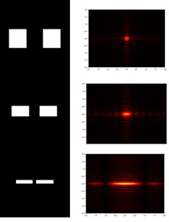
It can be observed that these circles are considered as circular apertures. Their Fourier transform is an Airy pattern. As the radius of the circular apertures increases, the Airy disc decreases in radius.

Square apertures and their FT modulus

Meanwhile, as the square aperture gets smaller, its FT widens. The gaussian aperture, on the other hand, has the same trend as the circular aperture except that, instead of varying the radius, we vary the variance.

Gaussian apertures and their FT modulus

It can be noted in the first two variances (0.1 and 0.2), the former resembles 2 dirac-deltas in space and the latter resembles 2 circular apertures along x-axis. This is the reason why the FT modulus of the first 2 gaussian apertures resemble the FT modulus of a dirac-delta and a circular aperture, respectively.


B. Inverse Fourier Transform

random points (left), arbitrary pattern (middle), Inverse Fourier Tranforn when the two are convolved (right)

When two images are convolved and their inverse Fourier transform are taken, the resulting image is just a product of the two images. The pattern adheres to the location of the dirac-deltas (dots). The image above shows how the Array Theorem works. When you a function and a dirac-delta, the functions will add linearly but shifted to an new location, depending on where the dirac-deltas are located.

original image (left) and FT of hte modulus (right)

The Fourier transform of the image on the left is the image on the right and vice-versa. As one increases the spacing in the original pattern, the spacing between the dots in the Fourier transform of the image is narrower.

C. Line Removal

Unwanted lines in a picture can be removed by creating a mask that filters these lines out.

(left to right) original image, FT of the image, mask, and masked image

In the final image, it can be observed that the visible lines have been removed.

D. Canvas Weave Modeling and Removal

(left to right) original cropped image, FT of the original cropped image, mask filter, result

After applying the mask, it can be seen that the weave pattern has been partly removed. Here is the Fourier transform of the inverted filter mask used.

Inverted mask filter (left) and its Fourier Transform (right)

The Fourier transform of the filter mask shows us the weave pattern in the painting that was removed. 

Despite the long hours of debugging, I enjoyed doing this activity. :)

Thus, I give myself a 13 for learning the techniques, applying what I have learned in my optics class and for patiently debugging my code until it gives the right results.

A big thanks to Eloi for the helpful discussions and to Mabel for helping me debug my code. :)