Enhancement in the Frequency Domain

I've been working with Fourier Transform since 3rd year. Back then, I didn't know that it would be one powerful transform that I would be using more often, be it in the field of image processing or signal processing.

This is one of those activities that really made me appreciate Fourier transform. Aside from its use on determining the frequencies in a signal, Fourier transform can also be used to enhance an image by blocking or putting a mask on unwanted frequencies.

A. Fourier Transform of Different Apertures

First, given two dots equally-spaced along the x-axis, applying Fourier transform would give you alternating dark and white bands. A dot is a representation of a dirac-delta.

Two dots symmetric along the x-axis and its FT modulus(left to right)

Two dots give you a cosine function in 2D as your Fourier transform. Replacing these dots with 2 circles give you an Airy pattern.

Circular Apertures and its FT modulus at varying radii

It can be observed that these circles are considered as circular apertures. Their Fourier transform is an Airy pattern. As the radius of the circular apertures increases, the Airy disc decreases in radius.

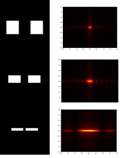
Square apertures and their FT modulus

Meanwhile, as the square aperture gets smaller, its FT widens. The gaussian aperture, on the other hand, has the same trend as the circular aperture except that, instead of varying the radius, we vary the variance.

Gaussian apertures and their FT modulus

It can be noted in the first two variances (0.1 and 0.2), the former resembles 2 dirac-deltas in space and the latter resembles 2 circular apertures along x-axis. This is the reason why the FT modulus of the first 2 gaussian apertures resemble the FT modulus of a dirac-delta and a circular aperture, respectively.


B. Inverse Fourier Transform

random points (left), arbitrary pattern (middle), Inverse Fourier Tranforn when the two are convolved (right)

When two images are convolved and their inverse Fourier transform are taken, the resulting image is just a product of the two images. The pattern adheres to the location of the dirac-deltas (dots). The image above shows how the Array Theorem works. When you a function and a dirac-delta, the functions will add linearly but shifted to an new location, depending on where the dirac-deltas are located.

original image (left) and FT of hte modulus (right)

The Fourier transform of the image on the left is the image on the right and vice-versa. As one increases the spacing in the original pattern, the spacing between the dots in the Fourier transform of the image is narrower.

C. Line Removal

Unwanted lines in a picture can be removed by creating a mask that filters these lines out.

(left to right) original image, FT of the image, mask, and masked image

In the final image, it can be observed that the visible lines have been removed.

D. Canvas Weave Modeling and Removal

(left to right) original cropped image, FT of the original cropped image, mask filter, result

After applying the mask, it can be seen that the weave pattern has been partly removed. Here is the Fourier transform of the inverted filter mask used.

Inverted mask filter (left) and its Fourier Transform (right)

The Fourier transform of the filter mask shows us the weave pattern in the painting that was removed. 

Despite the long hours of debugging, I enjoyed doing this activity. :)

Thus, I give myself a 13 for learning the techniques, applying what I have learned in my optics class and for patiently debugging my code until it gives the right results.

A big thanks to Eloi for the helpful discussions and to Mabel for helping me debug my code. :)

Histogram Manipulation

Since my first image of the Milky Way (which was last January this year), I've already been using the Curve Tool in Photoshop to enhance my image - make the Milky Way more visible. I was new to Photoshop then so I explored the software. It really amazed me how images looked much better after tweaking the Curve tool. But somehow, I thought I am only cheating because I am tweaking the curves.

Until the lesson we had on Histogram Manipulation...

The lesson actually fascinated me since it now explains how the Curve tool works and how is it possible to make details come out even when they are not there in the first place. Of course, since it is a really interesting topic for me, all ears on Ma'am Jing! =D

The image that I used is shown below. This was taken last January 2012 at Caliraya, Laguna. On site, another amateur astronomer (Kuya Irving) was teaching me how to do astrophotography. This was one of my first shots using the techniques I just learned then.

Image to be enhanced

The image was first converted to grayscale. The histogram and the normalized histogram or cumulative distribution function was then taken.

Grayscale version of the Original image

Histogram and the CDF of the original image

Here is the code used for the images above.

In order to manipulate the histogram, we need to use backprojection.

How are we going to do that?

Simple. Just like the Curve tool, we also need to tweak the CDF by introducing a desired CDF. Now, we start with the basic and very common one - a linear CDF. A linear CDF indicates that the white and black pixels are uniformly distributed.

First, we get the corresponding CDF, y1,  of x1. Then, find the value of the same CDF of the original image in your desired CDF, y2. Once found, check the corresponding x2 of y2. Replace x1 with x2. Do this for all values of the grayscale from 0 to 255.

Here is the code I used.

The algorith, for the code is shown as follows:

RESULTS


Linear:

Image after implementing a linear CDF

Histogram of the enhanced image using a linear CDF

A comparison of the desired CDF (left) and the resulting CDF (right)

 Quadratic:

Image after implementing a quadratic CDF

Histogram of the image above

A comparison of the desired CDF (left) and the resulting CDF (right)

The difference in the resulting images compared to the original is observable. It can be observed that histogram of the resulting images has shifted and that their CDF is either linear or quadratic in form but neither is smooth.

While this topic proved to be interesting and really useful, it may not seem really practical to other people since the process is quite "long" and "tedious". You need to have the correct function in order to get a really good enhanced image. Softwares such as Adobe Photoshop and Gimp provides the appropriate tool for image manipulation. 

Using Adobe Photoshop

Using Gimp

Here are sample enhanced images. These are my treasured Milky way shots and the only thing I tweaked to make the details come out is the Curves tool :)

Original Image 1

Enhanced Image 1

Original Image 2

Enhanced Image 2

There ya go! Image processing is really fun and interesting. Oh, how I wish we have more Image processing subjects.

Anyway, I give myself a 13. I really worked hard for this (because it took me a while before getting the right code and lots of editing). I would like to thank Mabelle for helping me understand the concept better and to Ate Jen's blog for making me see what went wrong in my code. :) Of course, thank you, Ma'am Jing, for simplifying things for us and for making the lessons as enjoyable as possible. :)

References:
1. Soriano, M. Image Enhancement by Histogram Manipulation 2010.
2. Manuel, J. Scilab Playground.

Area Segmentation

Hello, terminals! :) I am now a dual-OS user. hahaha! See!

Running Ubuntu on Windows

When I learned that the easiest way to get done with the activity is to install Scilab in Ubuntu, I was quite excited. I have never really used Ubuntu (except for those rare cases when the computer I was assigned to in the lab is run by Ubuntu). I am a Windows user ever since I learned about computers. I only learned about Ubuntu when I entered college. Loser much? =D

I seized the opportunity and asked a friend about the things I should know about Ubuntu. I asked him if I need to reformat my laptop so that I can have a dual boot. He is a Computer Science Major, he should know. He suggested that in order to save time (since reformatting laptops take long), I can use VMware Player. It's a virtual machine player. I can run any OS in VMware Player without needing to have a dual boot in my laptop. Cool! There were problems during the installation, at first, but I managed to run Ubuntu successfully in the virtual machine.

Next target: INSTALL SCILAB

I successfully installed Scilab using the Ubuntu Software Center. The version of Scilab that I installed is 5.2.2. Now, it's time to install SIP. My first attempts were unsuccessful. Google proved to be the best source of help during that time. I had to Google how to install SIP. I came across lots of tutorials but none proved to be successful. Until, I finally succumbed to the text file that tells the user the proper installation. I was really hesitant, at first. I'm not used to using terminals. Thanks again to Jerome for introducing me to the basic commands such as sudo, cd, ls and sudo apt-get install. It was quite confusing at first. Then, I realized I had no choice but to really learn it so I tried to play around. What seemed to be complex became interesting and fun, especially when you see lots of lines flashing on the terminal. Sometimes, it's frustrating if I get messages like "Permission deniend" or "Error". Nevertheless, the anticipation that the everything will work well (at the bottom line) was quite fun. So, for the successful installation of SIP, I used the terminal (since it also cannot be found in Ubuntu software center). Look, I am now using a terminal! 

Although this run failed, it was still amazing to see how the computer  processed my commands.

I downloaded SIP 0.5.6 from http://siptoolbox.sourceforge.net. I downloaded the source code. 

However, before installing the SIP toolbox, I must have properly installed AnImal (Animated Imaging Library), the image processing library of SIP. For AnImal to be properly installed, I must first have installed first ImageMagick. So, I first downloaded the AnImal 0.15.5  and ImageMagick 6.7.8 . I got them from the following site:

AnImal - http://animal.sourceforge.net

ImageMagick - www.imagemagick.org

First, I have to manually extract the ImageMagick file (it's in tar ball file). Inside the folder, look for Install-unix.txt and follow the instructions. In your terminal, make sure that you are in the directory in which the file is located. Here are commands for the installation:

./configure 

make

sudo make Install

make check

Once ImageMagick is successfully installed, install AnImal 0.5.15 using the same commands. 

After installing AnImal, you may now install SIP toolbox.

First, type this command "export PKG_CONFIG_PATH=/usr/local/lib/pkgconfig". Then compile and install SIP using the same commands you used for AnImal and ImageMagick installation. Once the installation is successfully done, type "make autoload" in order to load SIP to Scilab. And there you go! A successfully installed SIP toolbox in your Scilab. 

Of course, since I'm a newbie at installations like this, it took me three days to get everything right. But it was worth it! I can say that if not for those errors, I wouldn't learn how to properly use the terminals plus I've already learned basic Unix codes. Feels good to learn new things! :)

Since, I'm done with the installation. Let me now discuss how I did the activity.

Activity 4: Area Estimation

Test Images

First, I converted the images to black and white. Using the code below,

RGB to Black and White conversion Code

Since, I have already installed the SIP toolbox. I used the function follow () in order to get the contour of the images and the coordinates of the the contour. Here is the code I used:

In order to get the area of interest, Green's theorem was used. According to the theorem, an area of interest (with no concavities) is calculated by getting the summation of its pie slices.

Summation of the Pie slices is equal to the area

Green's Theorem

To implement the formula above, I used the the following code:

And to get the accuracy of the algorithm, the code below was used.

Algorithm accuracy checker code

The table below shows the results of the accuracy of my code.

Now, it's time to implement my code on area estimation.

My area of interest is the Quezon Memorial Circle. Here is its snapshot:

Quezon Memorial Circle

Post-processing was done using Paint. Here is the monochrome version of the image after post-processing.

Monochrome Image of the Map after Post-Processing

Snapshot of the Area tool and the calculated area

Using ratio and proportion, I found that 500m is equal to 107 pixels. I got the theoretical value of the land area from http://www.daftlogic.com/projects-google-maps-area-calculator-tool.htm.  Below is a tabulation of results.

The low percentage for accuracy can be attributed to the manual post-processing of the image and the defined area for the area tool for Google maps.

For this activity, I grade myself a 10 for learning Ubuntu and accomplishing the task at hand. :)



References:
1. Soriano, M. Area Estimation for Images with Defined Edges
2. theiszm.wordpress.com