Image Types and Formats

Pictures. Images. 

They tell you a story, be it sad, happy or enigmatic. But do you know what comprises a picture?

I haven't really thought about such things. I only see what my eyes see. I haven't really thought about the different image types or formats. I don't care if it's .jpg, .png or .bmp. As long as the image is saved, I'm done.

But I am thankful for a lecture on image types and formats. My knowledge on images now has depth. (haha!)

Well, you see, it's always fun to learn new things especially when they involve the things you see everyday. For me, the best way to test if you have really learned is to share it to other people and see if you can explain it to them with ease.

So, here I go. I' ll test how much I've learned.. Keep reading..

The types of images are divided into two. You have the basic and the advanced types. To better understand the types of images, I have attached pictures for you to see. :)

BASIC TYPES

1. Binary Type

An example of a Binary Image from photo.tutsplus.com

To get the some information about the image, you can just right click on the picture and select Properties. On the properties tab, click Details and there you'll see the image information. Here's a sample.

Image Properties for a Windows User

You can also get the image information using Scilab by typing imfinfo ('techo.jpg') to display their properties. A warning though, make sure the image you are trying to get the info from is in the current directory of Scilab console. If not, it might not open. Here's what I got when I used Scilab to display the properties.

Image Properties displayed using Scilab

2. Greyscale Image

Example of a Greyscale Image taken from 30 Stunning Examples
of Greyscale Photography at demortalz.com

3. Truecolor Images

One of my images during my parents' 21st anniversary

4. Indexed Image

The image of a parrot 

The palette of the image above

Photo courtesy of http://en.wikipedia.org/wiki/Indexed_color

ADVANCED IMAGE TYPE

1. High Dynamic Range (HDR) Image

One stormy day in the city - an HDR image

The image is taken from http://zowienews.com/2011/04/12/hdr-imagery-taking-the-country-by-storm

2. Multi or Hyperspectral Image

Satellite view of the world at night 

The image is taken from http://salz.soup.io/tag/World

3. 3D Image

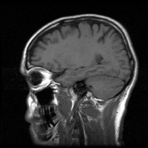
MRI scan of a human head

Image taken from mesotheliomasymptoms.com

4. Temporal images or videos

CONVERSION OF IMAGES

To convert the images from truecolor to grayscale, here is the Scilab code I used.

Code for Image conversion

Result of the Image conversion

USING THE HISTOGRAM

To get the histogram of the the scanned image in Activity 1, I used the following code.

Code for getting the histogram of the image

Histogram of the Grayscaled Image

Histogram of the Image with a bin width of 0.5

Since a threshold of 0.8 looks safe enough, here is the result.

On the left is the original image and on the right is the black and white image with a threshold of 0.8

Using the information obtained from the histogram, I was able to obtain the best threshold that would make the image look clearer than the original one as shown in the image above.

IMAGE FORMATS

1.  JPEG (Joint Photographic Expert Group)

           Image compression using JPEG can either be lossy (some information were lost) and lossless (all the information is preserved). The degree of compression can actually be adjusted depending on the file size that one wants. However, a smaller file size could mean an image with less quality.

2. BMP 

        The format is also know at bitmap image file. It can store 2D digital images.

3. GIF (Graphics Interchange format)

        This format is common in animations. It actually supports up to 8 bits per pixel. 

4. PNG (Portable Network Graphics)

        This format supports a lossless compression. This means that no information regarding the image is lost. However, since nothing is lost, the image file size could be quite big. This format only supports RGB color space.

5. TIFF (Tagged Image File Format)

       This format is good for storing images.

The source for the image formats is the Wikipedia. :)

Oh no! I'm afraid I'm running out of time. I think I just deserve an 8 for this since I was not able to fully explain the image formats. :( I made a huge mistake in this activity. Rather, I wasted my time processing images that were not needed for the activity and missed the ones that are really needed. 

I will really make sure I'll do better in the next activity. :)

Learning Scilab

At first, I was feeling lost. I had no idea, then, how to do the activity for the day. Panic consumed me when I learned that the deadline was by the end of the class. Scilab.. I am not really good at programming. Will I really learn Scilab in such a short time?


But, help from the heavens came. :)


Thanks to Ma'am Jing for giving us tips on how to start the activity and another thanks to my seatmates, Ash, Barts and Maine, for pointing out whatever I did wrong in my codes. These people saved my day! :)


So, here I am, feeling quite proud that the the day turned out well and I'm finally done with the activity. 


I will be posting here the codes that I used and the composite images I generated just to test different values for the different variables.


Centered Square Aperture


Code:



nx = 200; //number of elements along x and y
ny = 200; 
x = linspace(-1,1,nx); //range of x and y
y = linspace(-1,1,ny);
[X, Y] = ndgrid(x,y); //2D arrays of x and y
a = 0.1; // limit
A = zeros(nx,ny);
A (find(X < a & X > -a)) = 1;
A (find(Y < a & Y > -a)) = 1;
A (find(X < -a & Y < a)) = 0;
A (find(X < a & Y < -a)) = 0;
A (find(X > -a & Y > a)) = 0;
A (find(X > a & Y > -a)) = 0;
imshow (A);

Increasing centered square aperture

By increasing "a", the square aperture is also increasing. It still depends though on one's algorithm. 

Corrugated Roof


Code:

nx = 200; //number of elements along x and y
ny = 200; 
x = linspace(-1,1,nx); //range of x and y
y = linspace(-1,1,ny);
[X, Y] = ndgrid(x,y); //2D arrays of x and y


w = 100; //omega
y = sin(w*[Y]);
mesh(y);

Corrugated Roof at varying values for omega

As w or omega, which is equal to 2*pi*f, increases, the number of times the sinusoidal wave repeats in one cycle also increases. 


Grating along the X-direction


Code:



nx = 200; //number of elements along x and y
ny = 200; 
x = linspace(-1,1,nx); //range of x and y
y = linspace(-1,1,ny);
[X, Y] = ndgrid(x,y); //2D arrays of x and y



w = 100; // omega
y = sin(w*[Y]);
y = round(y);
imshow(y);

As omega increases, the number of alternating white and black bands, which are actually sinusoidal waves in 1D, also increases.




Annulus


Code:



nx = 200;
ny = 200;
x = linspace(-1,1,nx);
y = linspace(-1,1,ny);
[X, Y] = ndgrid(x,y);
r = sqrt(X.^2 + Y.^2); // radius
A = zeros(nx,ny);
A (find(r > 0.8)) = 1;
A (find(r > 1 )) = 0;
imshow (A);

Increasing Radius of the Annulus Aperture

Gaussian Transparency


Code:



nx = 200;
ny = 200;
x = linspace(-1,1,nx);
y = linspace(-1,1,ny);
[X, Y] = ndgrid(x,y);
r = sqrt(X.^2 + Y.^2);
A = zeros(nx,ny);
A (find(r < 0.5)) = 1;
F = fspecial('gaussian', hsize = [100,100], sigma = 0.5);
imf = imfilter(A, F);
imshow(imf);

Gaussian Transparency at Different Values for Sigma

The sigma dictates how transparent the aperture (white circle) will be. Increasing the sigma also increases the transparency. However, at very large values for sigma, such as 10000, there isn't a really observable change if we compare it to the transparency when sigma is 1000. 


I find the activity interesting and quite enjoyable. It was fun tweaking values and waiting for surprise changes in the images. Other interesting apertures can be formed depending on your parameters. 


For this activity, I give myself a 10. =p


Can't wait for the next image processing topics. :)

Digital Scanning

Yesterday, I was trying to figure out how to relate pixel location to real variables. The idea seemed familiar to me but I just can't remember. I had different solutions but they don't fit. In desperation, I asked Mabelle for some tips. She told me to use linear regression. She already had results and I have nothing. I was tempted to use programming but I hesitated. I am not that confident. While Mabelle was explaining to me the idea (how to solve the problem), it suddenly clicked to me that this was the very first thing Kirby taught me when I was in 3rd year. So, I immediately looked for my research notebook and there it is. Kirby's handwriting on my notebook. We already did this 2 years ago for the camera sensitivity experiment. My short-term amnesia is over. I can now perfectly remember how I did it 2 years ago. Thank you, Mabelle and Kirby for this. :)

So, here's how I did it.

1. Get the pixel location of the origin, x-coordinates and the y-coordinates. Write them down in Excel.
2. Make a table. One for the x-coordinates of the real and the pixel location in x and another one for the y-coordinates of the real and the pixel location in y.
3. Separately, graph the values. For my case, in the x-coordinate part of the image, my x was the pixel location and my y is the real values in the x-coordinate of the image. The same thing was done for the the Y-coordinate.

Displayed below are the graph, the equation and the R-squared value of the X and Y coordinates of the image.

4. Now, get the pixel location of points in the graph of the image. For my case, I took 60 points.
5. Using these points, insert the x and y value of points in the graph of the images to your equation in the X-coordinates. Then, using the same 60 points, do it also for the y-coordinates.
6. Once you have the value for the X and Y, graph these values.
7. Overlay the graph to the original image. Adjust the graph so that the x and y coordinates coincide.
8. See if you're able to perfectly reconstruct the original graph.

Here's what I got:

My best fit of the original graph

A small offset will result to a perfect reconstructed graph

It is not perfectly fit but it has the same shape as the original graph. This is the result after my 7th trial. The more points there are, the better the fit.

This skill is basic but very useful especially in preserving very old manuscripts. This activity made me realize something very important for a researcher: never forget everything that you have learned and always take notes of everything that you did in your experiment so as not to forget them the next time they are needed.

Because I took the points manually, I had to be very careful - a skill I don't usually possess but needed in research.

I think I just had a good start of the semester because of this activity. This activity slapped me hard in the face just to remind me that I should never forget everything that I learned and passed on to me in research. A helpful way to start my thesis year. :)


For this activity, I rate myself an 8 for doing my best despite the fact that I was not able to think of the solution to the problem on my own. Anyway, this is just the first. I'll improve next time. :)


The original graph used was from the PhD Dissertation in Physics of Minella C. Alarcon entitled Optical Remote Sensing using Low-Loss Optical Fiber Link in the Near Infrared Region last 1986.